Community

A summary of the demographic information of the NumPy survey respondents.

Show code cell source Hide code cell source

fname = "data/2021/numpy_survey_results.tsv"
column_names = [
    'age', 'gender', 'lang', 'lang_other', 'country', 'degree', 'degree_other',
    'field_of_study', 'field_other', 'role', 'role_other', 'version', 'version_other',
    'primary_use', 'share_code', 'programming_exp', 'numpy_exp', 'use_freq', 'components',
    'use_c_ext', 'prog_lang', 'prog_lang_other', 'surv2020'
]
demographics_dtype = np.dtype({
    "names": column_names,
    "formats": ['<U600'] * len(column_names),
})

data = np.loadtxt(
    fname, delimiter='\t', skiprows=3, dtype=demographics_dtype, 
    usecols=list(range(11, 33)) + [90], comments=None, encoding='UTF-16'
)

glue('2021_num_respondents', data.shape[0], display=False)

Demographics

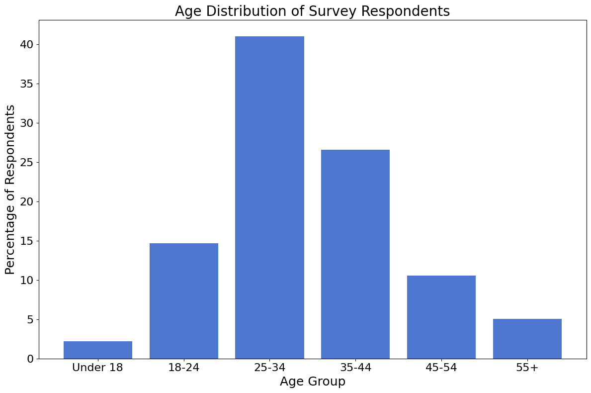
Age

Of the 522 survey respondents, 456 (87%) shared their age.

The majority of respondents are in the age groups 25-34 and 35-44. Very few respondents are older than 55, and even fewer are younger than 18.

Show code cell source Hide code cell source

# Ignore empty fields and "prefer not to answer"
drop = np.logical_and(data['age'] != '', data['age'] != 'Prefer not to answer')
age = data['age'][drop]
labels, cnts = np.unique(age, return_counts=True)
ind = np.array([5,0,1,2,3,4])
labels, cnts = labels[ind], cnts[ind]

fig, ax = plt.subplots(figsize=(12, 8))
ax.bar(
  np.arange(len(labels)),
  100 * cnts / age.shape[0], 
  tick_label=labels,
)
ax.set_ylabel('Percentage of Respondents')
ax.set_xlabel('Age Group')
ax.set_title("Age Distribution of Survey Respondents");
fig.tight_layout()

glue('2021_num_age_respondents', gluval(age.shape[0], data.shape[0]), display=False)

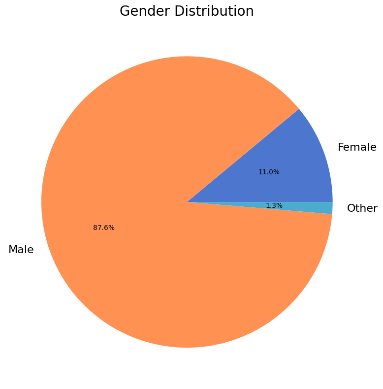
Gender

Of the 522 survey respondents, 453 (87%) shared their gender.

An majority of respondents identify as male. Only about 11% of respondents identify as female.

Show code cell source Hide code cell source

# Ignore empty fields and "prefer not to answer"
drop = np.logical_and(data['gender'] != '', data['gender'] != 'Prefer not to answer')
gender = data['gender'][drop]
labels, cnts = np.unique(gender, return_counts=True)

fig, ax = plt.subplots(figsize=(8, 8))
ax.pie(cnts, labels=labels, autopct='%1.1f%%')
ax.set_title("Gender Distribution");
fig.tight_layout()

glue('2021_num_gender', gluval(gender.shape[0], data.shape[0]), display=False)

Language Preference

Of the 522 respondents, 497 (95%) shared their preferred language.

Over 67% of respondents reported English as their preferred language.

Show code cell source Hide code cell source

# Ignore empty fields
lang = data['lang'][data['lang'] != '']
# Self-reported language
lang_other = data['lang_other'][data['lang_other'] != '']
lang_other = capitalize(lang_other)
lang = np.concatenate((lang, lang_other))
labels, cnts = np.unique(lang, return_counts=True)
cnts = 100 * cnts / cnts.sum()
I = np.argsort(cnts)[::-1]
labels, cnts = labels[I], cnts[I]

# Create a summary table
with open('_generated/language_preference_table.md', 'w') as of:
    of.write('| **Language** | **Preferred by % of Respondents** |\n')
    of.write('|--------------|-----------------------------------|\n')
    for lbl, percent in zip(labels, cnts):
        of.write(f'| {lbl} | {percent:1.1f} |\n')

glue('2021_num_lang_pref', gluval(lang.shape[0], data.shape[0]), display=False)

Click to show/hide table

Language	Preferred by % of Respondents
English	67.2
Other	6.6
Spanish	6.2
French	5.4
Japanese	5.0
Russian	1.8
German	1.4
Mandarin	1.0
Portuguese	0.6
Polish	0.6
Swedish	0.4
Czech	0.4
Italian	0.4
Turkish	0.4
Chinise	0.2
中文	0.2
Chinese	0.2
Bulgarian	0.2
Allemand	0.2
Hungarian	0.2
Dutch	0.2
Hebrew	0.2
Hindi	0.2
Indonesian	0.2
Korean	0.2
“norwegian “	0.2

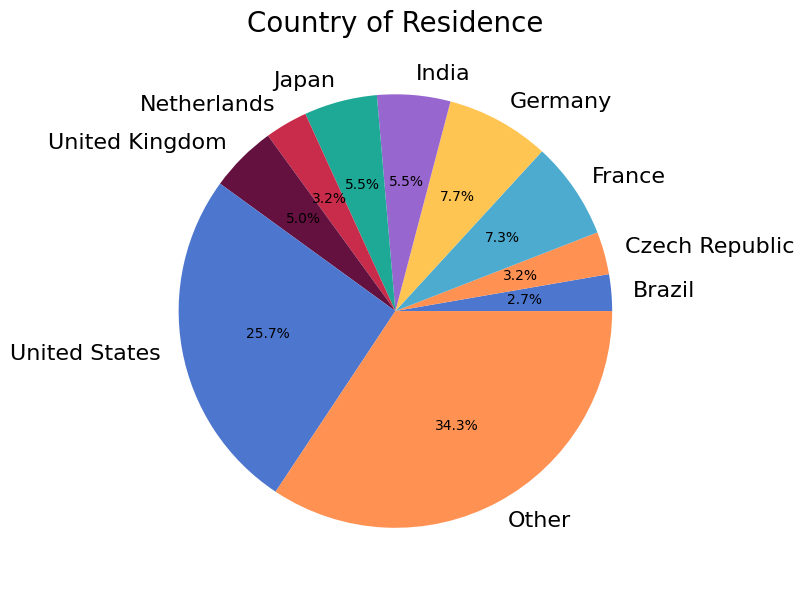
Country of Residence

Of the 522 respondents, 440 (84%) shared their current country of residence. The survey saw respondents from 54 countries in all. A quarter of respondents reside in the United States.

The following chart shows the relative number of respondents from ~10 countries with the largest number of participants. For privacy reasons, countries with fewer than a certain number of respondents are not included in the figure, and are instead listed in the subsequent table.

Show code cell source Hide code cell source

# Preprocess data
country = data['country'][data['country'] != '']
country = strip(country)
# Distribution
labels, cnts = np.unique(country, return_counts=True)
# Privacy filter
num_resp = 10
cutoff = (cnts > num_resp)
plabels = np.concatenate((labels[cutoff], ['Other']))
pcnts = np.concatenate((cnts[cutoff], [cnts[~cutoff].sum()]))

# Plot
fig, ax = plt.subplots(figsize=(8, 8))
ax.pie(pcnts, labels=plabels, autopct='%1.1f%%')
ax.set_title("Country of Residence");
fig.tight_layout()

# Map countries to continents
import pycountry_convert as pc
cont_code_to_cont_name = {
    'NA': 'North America',
    'SA': 'South America',
    'AS': 'Asia',
    'EU': 'Europe',
    'AF': 'Africa',
    'OC': 'Oceania',
}
def country_to_continent(country_name):
    cc = pc.country_name_to_country_alpha2(country_name)
    cont_code = pc.country_alpha2_to_continent_code(cc)
    return cont_code_to_cont_name[cont_code]
c2c = np.vectorize(country_to_continent, otypes='U')

# Organize countries below the privacy cutoff by their continent
remaining_countries = labels[~cutoff]
continents = c2c(remaining_countries)
with open('_generated/countries_by_continent.md', 'w') as of:
    of.write('|  |  |\n')
    of.write('|---------------|-------------|\n')
    for continent in np.unique(continents):
        clist = remaining_countries[continents == continent]
        of.write(f"| **{continent}:** | {', '.join(clist)} |\n")

glue('2021_num_unique_countries', len(labels), display=False)
glue(
    '2021_num_country_respondents',
    gluval(country.shape[0], data.shape[0]),
    display=False
)

Africa:	Egypt, Ghana, Kenya, Nigeria, South Africa, Zimbabwe
Asia:	Bangladesh, China, Indonesia, Israel, Malaysia, Pakistan, Singapore, South Korea, Turkey
Europe:	Austria, Belgium, Bulgaria, Denmark, Finland, Hungary, Iceland, Ireland, Italy, Latvia, Norway, Poland, Russia, Slovakia, Spain, Sweden, Switzerland, Ukraine
North America:	Canada, Cuba, Mexico
Oceania:	Australia, Vanuatu
South America:	Argentina, Chile, Colombia, Ecuador, Paraguay, Peru, Venezuela

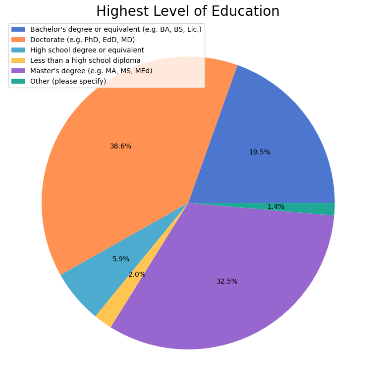
Education

440 (84%) respondents shared their education history, spanning the range from pre-highschool graduation through Doctorate level with many other specialist degrees.

Generally, respondents are highly educated. Nine out of ten have at least a Bachelor’s degree and one in three holds a PhD.

The following figure summarizes the distribution for the highest degrees obtained by respondents.

Show code cell source Hide code cell source

degree = data['degree'][data['degree'] != '']
labels, cnts = np.unique(degree, return_counts=True)

fig, ax = plt.subplots(figsize=(8, 8))
ax.pie(cnts, labels=labels, autopct='%1.1f%%', labeldistance=None)
ax.legend()
ax.set_title("Highest Level of Education");
fig.tight_layout()

glue('2021_num_education', gluval(degree.shape[0], data.shape[0]), display=False)

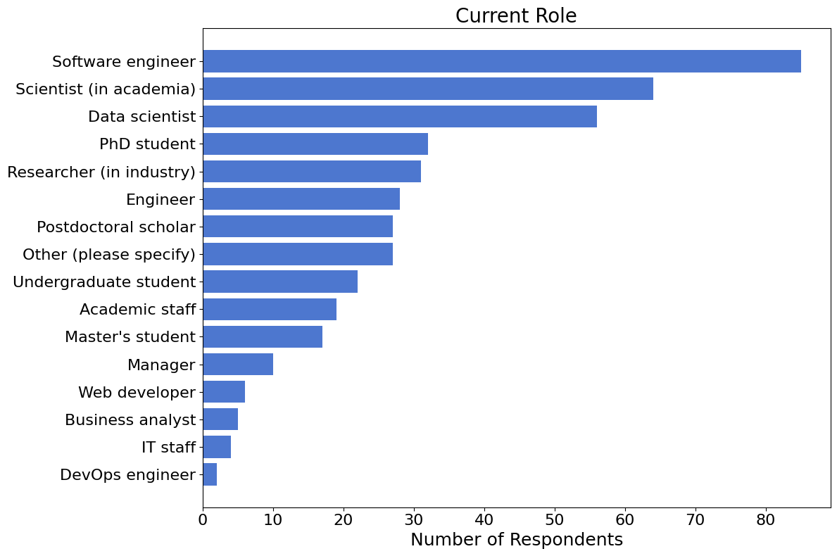
Job Roles

205 (47%) of the 435 respondents who shared their occupation identify as an Data scientist, Scientist (in academia), or Software engineer.

Show code cell source Hide code cell source

role = data['role'][data['role'] != '']
labels, cnts = np.unique(role, return_counts=True)

# Sort results by number of selections
inds = np.argsort(cnts)
labels, cnts = labels[inds], cnts[inds]

fig, ax = plt.subplots(figsize=(12, 8))
ax.barh(np.arange(len(cnts)), cnts, align='center')
ax.set_yticks(np.arange(len(cnts)))
ax.set_yticklabels(labels)
ax.set_xlabel("Number of Respondents")
ax.set_title("Current Role");
fig.tight_layout()

glue('2021_num_occupation', role.shape[0], display=False)
glue(
    '2021_num_top_3_categories',
    gluval(cnts[-3:].sum(), role.shape[0]),
    display=False,
)
glue('2021_top_3_categories', f"{labels[-3]}, {labels[-2]}, or {labels[-1]}", display=False)

Show code cell source Hide code cell source

# Ignore empty fields and "prefer not to answer"
drop = np.logical_and(data['surv2020'] != '', data['surv2020'] != 'Not sure')
surv2020 = data['surv2020'][drop]
labels, cnts = np.unique(surv2020, return_counts=True)

glue('2021_num_surv2020_respondents', gluval(surv2020.shape[0], data.shape[0]), display=False)
yes_percent = 100 * cnts[1].sum() / cnts.sum()
glue('2021_yes_percent', f"{yes_percent:1.1f}", display=False)

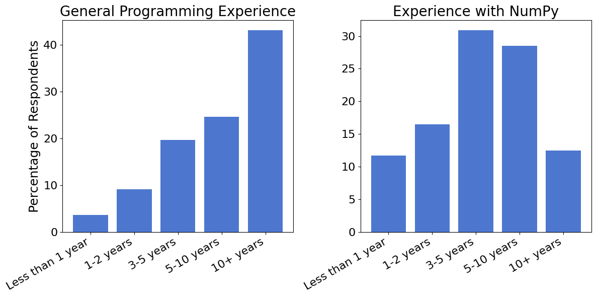
Experience and Usage

Programming Experience

68% of respondents have significant experience in programming, with veterans (10+ years) taking the lead. Interestingly, when it comes to using NumPy, noticeably more of our respondents identify as beginners than experienced users.

Show code cell source Hide code cell source

fig, axes = plt.subplots(1, 2, figsize=(12, 6))
# Ascending order for figure
ind = np.array([-1, 0, 2, 3, 1])
for exp_data, ax in zip(('programming_exp', 'numpy_exp'), axes):
    # Analysis
    prog_exp = data[exp_data][data[exp_data] != '']
    labels, cnts = np.unique(prog_exp, return_counts=True)
    cnts = 100 * cnts / cnts.sum()
    labels, cnts = labels[ind], cnts[ind]
    # Generate text on general programming experience
    glue(f'2021_{exp_data}_5plus_years', f"{cnts[-2:].sum():2.0f}%", display=False)
    # Plotting
    ax.bar(np.arange(len(cnts)), cnts)
    ax.set_xticks(np.arange(len(cnts)))
    ax.set_xticklabels(labels)
axes[0].set_title('General Programming Experience')
axes[0].set_ylabel('Percentage of Respondents')
axes[1].set_title('Experience with NumPy');
fig.autofmt_xdate();
fig.tight_layout();

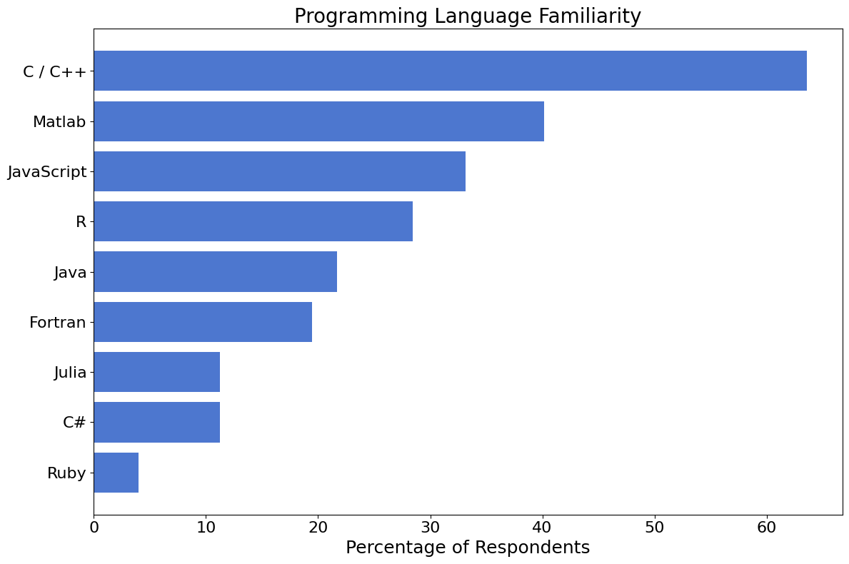
Programming Languages

401 (77%) of survey participants shared their experience with other programming languages. 64% of respondents are familiar with np.str_(‘C / C++’), and 40% with np.str_(‘Matlab’).

Show code cell source Hide code cell source

pl = data['prog_lang'][data['prog_lang'] != '']
num_respondents = len(pl)
glue('2021_num_proglang_respondents', gluval(len(pl), data.shape[0]), display=False)

# Flatten & remove 'Other' write-in option
other = 'Other (please specify, using commas to separate individual entries)'
apl = []
for row in pl:
    if 'Other' in row:
        row = ','.join(row.split(',')[:-2])
        if len(row) < 1:
            continue
    apl.extend(row.split(','))
labels, cnts = np.unique(apl, return_counts=True)
cnts = 100 * cnts / num_respondents
I = np.argsort(cnts)
labels, cnts = labels[I], cnts[I]

fig, ax = plt.subplots(figsize=(12, 8))
ax.barh(np.arange(len(cnts)), cnts, align='center')
ax.set_yticks(np.arange(len(cnts)))
ax.set_yticklabels(labels)
ax.set_xlabel("Percentage of Respondents")
ax.set_title("Programming Language Familiarity")
fig.tight_layout()

# Highlight two most popular
glue('2021_num_top_lang', f"{cnts[-1]:2.0f}%", display=False)
glue('2021_top_lang', labels[-1], display=False)
glue('2021_num_2nd_lang', f"{cnts[-2]:2.0f}%", display=False)
glue('2021_second_lang', labels[-2], display=False)

84 (21%) percent of respondents reported familiarity with computer languages other than those listed above. Of these, Rust was the most popular with 17 (4%) respondents using this language. A listing of other reported languages can be found below (click to expand).

Show code cell outputs Hide code cell outputs

['"' '"cobol' '"tcl' '-' 'amigae' 'asembler mc68k' 'asembler x86'
 'assembly' 'awk' 'bash' 'basic' 'clojure' 'cython' 'dart' 'dpl' 'elixir'
 'elm' 'f#' 'forth' 'go' 'golang' 'haskel' 'haskell' 'idl' 'kotlin' 'lisp'
 'llvm ir' 'logo' 'lua' 'mathematica' 'matlab' 'mysql' 'nim' 'nim lang'
 'nix' 'none' 'none except python' 'objective-c' 'ocaml' 'pascal' 'perl'
 'php' 'prolog' 'python' 'rust' 'scala' 'scheme' 'shell' 'sql' 'stata'
 'swift' 'systemverilog' 't-sql' 'tcl' 'tcl/tk' 'tex' 'typescript' 'vba'
 'verilog' 'visual basic' 'visual foxpro' 'what does familiar mean?'
 'wolfram']

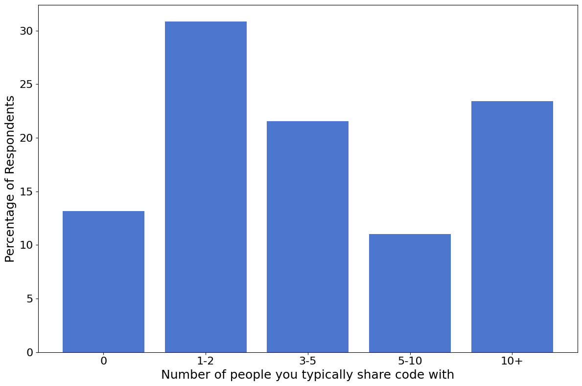
Code Sharing

418 (80%) of survey participants shared information on how many others they typically share code with. Most respondents share code with 1-2 people.

Show code cell source Hide code cell source

from numpy_survey_results.utils import flatten

share_code = data['share_code'][data['share_code'] != '']
labels, cnts = np.unique(flatten(share_code), return_counts=True)

# Sort categories in ascending order (i.e. "0", "1-2", "3-5", "5-10", "10+")
ind = np.array([0, 1, 3, 4, 2])
labels, cnts = labels[ind], cnts[ind]

fig, ax = plt.subplots(figsize=(12, 8))
ax.bar(
    np.arange(len(labels)),
    100 * cnts / share_code.shape[0], 
    tick_label=labels,
)
ax.set_ylabel('Percentage of Respondents')
ax.set_xlabel('Number of people you typically share code with')
fig.tight_layout()

# Highlights most popular
glue('2021_top_share', str(labels[np.argmax(cnts)]), display=False)

# Number who answered question
glue(
    '2021_num_share_code',
    gluval(share_code.shape[0], data.shape[0]),
    display=False
)