numpy.random.Generator.zipf
method
-
Generator.zipf(a, size=None)¶ Draw samples from a Zipf distribution.
Samples are drawn from a Zipf distribution with specified parameter a > 1.
The Zipf distribution (also known as the zeta distribution) is a continuous probability distribution that satisfies Zipf’s law: the frequency of an item is inversely proportional to its rank in a frequency table.
- Parameters
- a
floator array_like of floats Distribution parameter. Must be greater than 1.
- size
intortupleof ints, optional Output shape. If the given shape is, e.g.,
(m, n, k), thenm * n * ksamples are drawn. If size isNone(default), a single value is returned ifais a scalar. Otherwise,np.array(a).sizesamples are drawn.
- a
- Returns
- out
ndarrayor scalar Drawn samples from the parameterized Zipf distribution.
- out
See also
scipy.stats.zipfprobability density function, distribution, or cumulative density function, etc.
Notes
The probability density for the Zipf distribution is

where
 is the Riemann Zeta function.
It is named for the American linguist George Kingsley Zipf, who noted that the frequency of any word in a sample of a language is inversely proportional to its rank in the frequency table.
References
- 1
Zipf, G. K., “Selected Studies of the Principle of Relative Frequency in Language,” Cambridge, MA: Harvard Univ. Press, 1932.
Examples
Draw samples from the distribution:
>>> a = 2. # parameter
>>> s = np.random.default_rng().zipf(a, 1000)
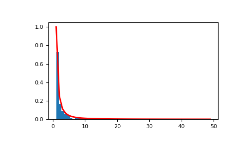
Display the histogram of the samples, along with the probability density function:
>>> import matplotlib.pyplot as plt
>>> from scipy import special
Truncate s values at 50 so plot is interesting:
>>> count, bins, ignored = plt.hist(s[s<50],
...         50, density=True)
>>> x = np.arange(1., 50.)
>>> y = x**(-a) / special.zetac(a)
>>> plt.plot(x, y/max(y), linewidth=2, color='r')
>>> plt.show()